Stable Diffusion Series 4/5 - Variational Auto-Encoders
Why do we need an auto-encoder for Stable Diffusion ?
The Need for Efficient Data Representations
Imagine I give you two number sequences and ask which one is easier to remember:
- Sequence A - 3, 7, 12, 19, 24
- Sequence B - 1, 3, 5, 7, 9, 11, 13, 15, 17, 19, 21, 23, 25, 27, 29
Although Sequence A has fewer numbers, each one is unique and independent. You’d have to remember each number individually. On the other hand, while Sequence B is longer, it follows a simple pattern: it’s the sequence of odd numbers from 1 to 29. This pattern makes it much easier to remember because instead of memorizing all 15 numbers, you only need to store the starting number (1), the ending number (29), and the rule (“odd numbers”).
This analogy highlights the concept of efficient data representations. Instead of storing or processing all the details of the data, we seek a compact and structured way to capture the essential features, reducing redundancy and preserving the key information. This is especially useful when dealing with high-dimensional data like images, audio, or text. Efficient representations enable models to focus on meaningful patterns and relationships within the data, leading to better performance in tasks such as classification, clustering, and generation.
What Are Autoencoders?
Autoencoders are a type of neural network architecture designed to learn efficient data representations in an unsupervised manner. Unlike supervised learning, where models learn to map inputs to specific outputs, autoencoders learn to encode the input data into a compressed form and then decode it back to reconstruct the original input. This process helps them identify and retain the most critical features while discarding irrelevant information.
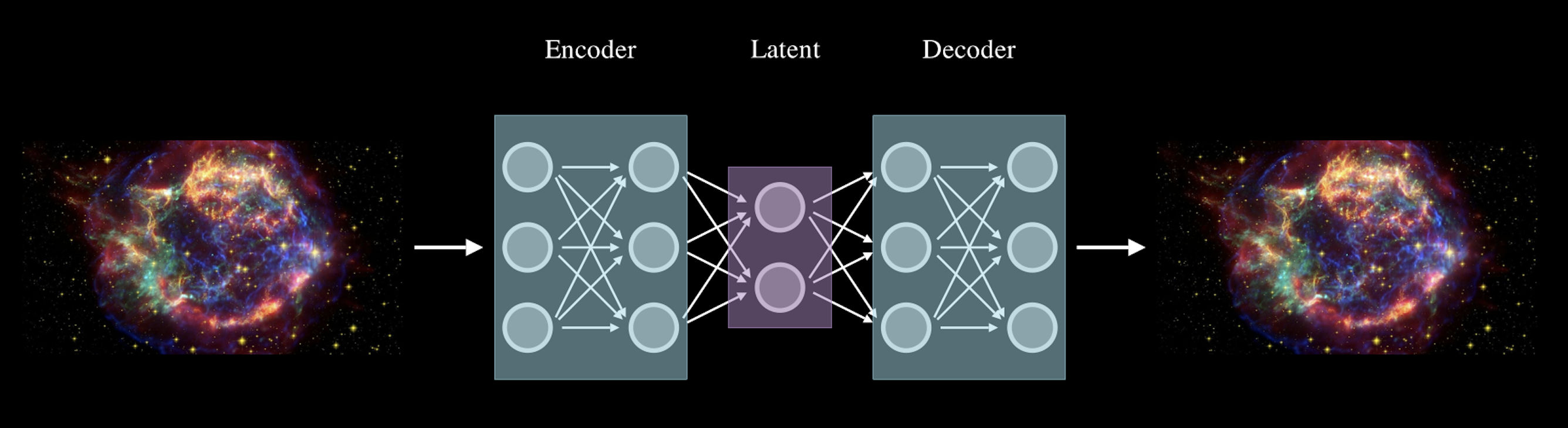
The architecture of a basic autoencoder consists of two main parts:
- Encoder - The encoder compresses the input data into a lower-dimensional space known as the latent representation. This compression forces the network to learn the essential characteristics of the input data and discard the less significant details.
- Decoder - The decoder takes the latent representation and reconstructs it back to match the original input as closely as possible. This reconstruction step ensures that the encoder has effectively captured the underlying structure of the input data.
Visually, autoencoders resemble a typical neural network with an input layer, hidden layers, and an output layer. However, unlike other neural networks, the number of neurons in the output layer of an autoencoder must be equal to the number of inputs to ensure it can reconstruct the original data.
Since the latent representation has a lower dimensionality than the input data, the network is unable to simply copy the input features into the latent space. Instead, it’s forced to learn the most salient features and representations that summarize the input. This makes autoencoders highly efficient at dimensionality reduction and feature extraction.
Moreover, autoencoders can be used as generative models. By training on a given dataset, they learn to generate new data samples that resemble the original training data.
Convolutional Autoencoders
In our previous discussions on images, we highlighted how convolutional layers are more effective than dense layers for capturing spatial hierarchies and local features. When building autoencoders for images, it’s beneficial to use Convolutional Autoencoders (CAEs) instead of fully connected ones. This allows us to leverage the strengths of convolutional operations, such as detecting edges, textures, and shapes, while preserving spatial structure.
But rest assured, the core architecture—comprising the encoder, latent representation, and decoder—remains the same with some minor modifications. The key difference is how these components are constructed:
- Encoder - The encoder in a convolutional autoencoder is similar to that of a standard CNN. It consists of a series of convolutional and pooling layers (or downsampling layers). As with a typical CNN, the purpose of the encoder is to progressively reduce the height and width of the image while increasing its depth, meaning it transforms the original image into a set of lower-dimensional feature maps. These feature maps capture the key patterns and spatial structures of the image in a compact form.
- Decoder - The decoder reverses the transformations applied by the encoder. It uses upsampling layers (like transposed convolutions or interpolation layers) to gradually increase the height and width of the feature maps while reducing their depth, reconstructing the input image. The objective is to restore the image’s original dimensions and structure as accurately as possible, based on the compressed latent representation.
For now, we won’t delve into the implementation details until we cover the theoretical aspects more thoroughly. However, later in this chapter, we’ll show how convolutional autoencoders can be tailored for more complex tasks such as Stable Diffusion. In fact, Stable Diffusion uses convolutional autoencoders as part of its architecture. We’ll explore how and why these models are used in greater detail as we proceed.
Variational Autoencoders
Variational Autoencoders (VAEs) are one of the most widely used and popular types of autoencoders, introduced in the paper
The VAE plays a crucial role in diffusion model architecture. The encoder produces the latent representation of an input image, in the case of image-to-image, or a noisy input in the case of text-to-image, while the decoder is the final step that reconstructs and outputs the image you requested with a text prompt.
The key distinction between a VAE and a standard autoencoder is that instead of mapping the input to a fixed latent vector, VAEs aim to map it to a distribution. More precisely, the latent vector is replaced by two components: the mean \(\mu\) and the standard deviation \(\sigma\). From this Gaussian distribution, defined by \(\mu\) and \(\sigma\), we sample a latent vector, which is then passed to the decoder to reconstruct the input, just like in traditional autoencoders. This leads to two important characteristics of VAEs:
- Probabilistic Nature - The latent space of VAEs is probabilistic, meaning that each time we sample from the Gaussian distribution, we get slightly different latent representations. As a result, the output of the decoder is also probabilistic, introducing variability in the reconstructions.
- Generative Capabilities - Because of their stochastic nature, VAEs are generative models. They can generate new instances that look similar to the data they were trained on but are, in fact, unique. For example, if a VAE is trained on images of dogs, it could generate a new image of a dog that resembles the training data but includes subtle variations, like a dog with three ears. These new samples come from the same underlying distribution as the training data but introduce novel variations.
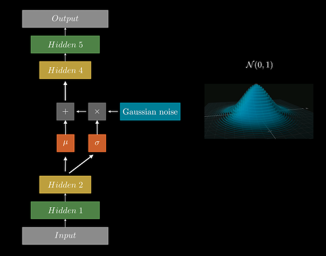
As illustrated in the diagram above, after the encoder processes the input, the final layer of the encoder outputs two vectors: \(\mu\) and \(\sigma\) of the latent distribution. Instead of directly sampling from these vectors, an additional step is introduced — the reparameterization trick.
The Reparameterization Trick
In the ideal scenario, we would sample directly from the latent distribution using the computed \(\mu\) and \(\sigma\). However, during training, we use backpropagation to compute the gradient of the loss with respect to every trainable parameter in the network. The stochastic nature of \(\mu\) and \(\sigma\) creates a problem here, as the gradients cannot propagate through the sampling step.
The solution is the reparameterization trick, which introduces a clever workaround: Instead of sampling directly from the Gaussian distribution defined by \(\mu\) and \(\sigma\), we transform the process into something more manageable for backpropagation. Here’s how it works:
- We sample an auxiliary variable \(\epsilon\) from a standard normal distribution with \(\mu = 0\) and \(\sigma = 1\).
- The latent vector is then computed as \(z=μ+σ\ast \epsilon\). This operation allows the mean and standard deviation to remain deterministic, which makes them suitable for gradient-based learning. The stochastic aspect is now captured by \(\epsilon\).
By using this trick, we move the randomness into a non-trainable node \(\epsilon\) while keeping \(\mu\) and \(\sigma\) as trainable parameters, allowing gradients to flow during backpropagation.
Why Not Train \(\epsilon\)?
A common question might arise: “Why not train \(\epsilon\)?” The answer is simple — \(\epsilon\) is sampled fresh in every forward pass, acting as a fixed noise source. Its role is to introduce controlled randomness, and it doesn’t need to be learned since it always comes from the standard Gaussian distribution (mean 0, standard deviation 1).
VAE Equation
Now that we’ve covered how VAEs differ from traditional autoencoders, let’s dive deeper into their loss function. The VAE loss combines two important components that work together to ensure the model can generate new data while keeping the latent space well-organized.
Below is the general formula for the VAE loss:
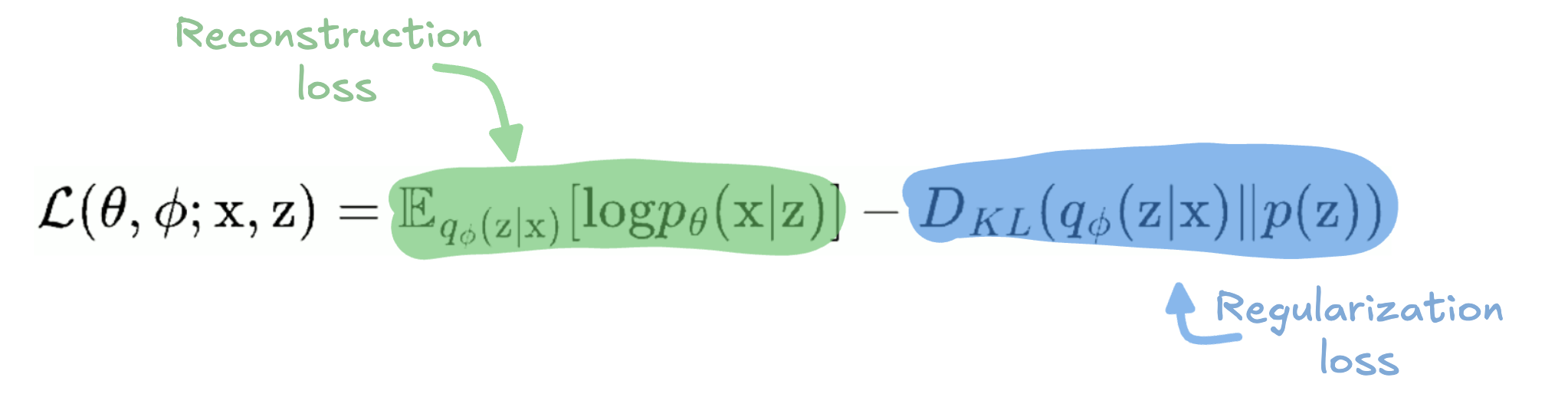
It consists of two parts:
- Reconstruction Loss - The first term helps the model recreate the input data as accurately as possible.
- Regularization Loss - The second term, also known as the Kullback-Leibler (KL) divergence, penalizes the model if the latent space deviates too much from the normal distribution.
Let’s break these components down further.
Reconstruction Loss
The primary goal of the VAE is to take an input (e.g., an image), encode it into a simpler latent representation, and then decode it to reconstruct the original input. The reconstruction loss measures how close the reconstructed output is to the original input.
To make this clearer: Suppose you give the model a picture of a cat. The model compresses the image into a latent vector and then reconstructs it. The reconstruction loss checks how similar the new image is to the original. The more accurate the reconstruction, the smaller this loss becomes.
Technically, this term is the likelihood of the original input \(x\) given the latent representation \(z\) from the encoder. We aim to maximize this likelihood so that the decoder, represented by \(p_\theta(x∣z)\), can generate data as close as possible to the original input, which was compressed by the encoder \(q_\phi(z∣x)\).
Regularization Loss
The second part of the VAE loss function is the regularization term, which is where the probabilistic nature of VAEs comes into play. Recall that the encoder doesn’t output a single deterministic latent vector but instead generates a mean \(\mu\) and standard deviation \(\sigma\), allowing us to sample from a Gaussian distribution to create the latent representation.
This stochastic property adds flexibility, allowing the VAE to generate smooth, continuous variations of new data. However, to ensure that the latent space is well-structured and meaningful, we need to regularize it. This is achieved through the KL divergence, which measures how much the learned latent distribution, produced by the encoder, deviates from a standard Gaussian distribution. The goal is to make the latent vectors follow this normal distribution so that similar inputs produce similar latent representations. If the latent space is poorly organized — i.e., if latent vectors are scattered randomly — generating new, coherent data points would be difficult. The KL divergence penalizes the model when the latent vectors stray too far from the Gaussian distribution, encouraging a well-organized and continuous latent space.
In summary, the regularization term ensures that the latent space remains structured, preventing it from becoming chaotic, and helping the model generate meaningful and smooth variations from the training data.
Residual Blocks
Residual blocks, or skip connections, were a game-changing innovation introduced in the ResNet paper
So, what was going wrong? As networks became deeper, they struggled to learn optimal weights. Information struggles to pass through all the layers, and the gradients during backpropagation became increasingly small, leading to what’s known as the vanishing gradient problem. This made it difficult for the network to update weights, especially in the earlier layers, causing deep models to underperform compared to shallower ones.
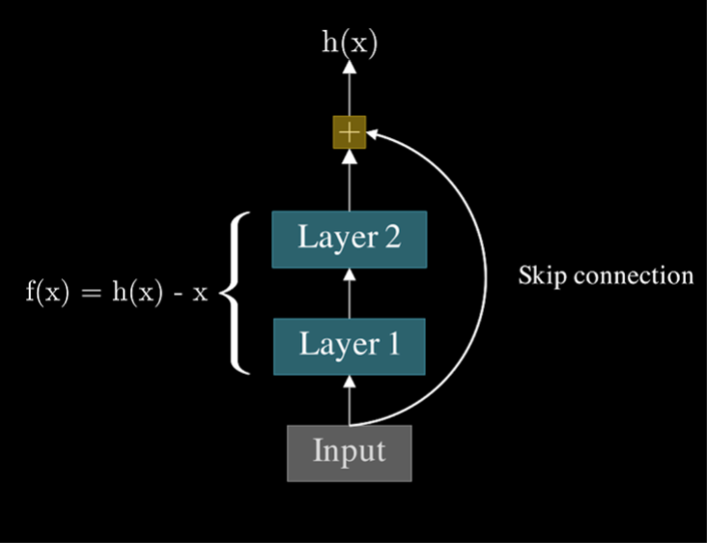
Residual blocks provided a clever solution to this problem. Rather than forcing the network to directly learn the full mapping \(f(x)\), residual blocks allow the network to learn the residual \(h(x)=f(x)-x\), which simplifies to \(f(x)=h(x)+x\). The key is an identity connection — a shortcut — that bypasses one or more layers, letting information skip through the network without obstruction. This allows gradients to flow more freely during backpropagation, addressing the vanishing gradient issue.
But the benefits of residual blocks don’t stop there. These identity connections also speed up training. Early in training, when weights are initialized near zero, approximating the identity function provides a helpful kickstart. In traditional networks, some layers may struggle to “wake up” because of small gradients or poor initialization. But with residual blocks, the model can start by learning the identity function \(f(x)\approx x\) , which allows it to make rapid initial progress before moving on to learn more complex mappings. This ensures that the model doesn’t get stuck early on, making learning faster and more efficient.
Now, you might wonder: why are residual blocks important in the context of stable diffusion? In architectures like Stable Diffusion, residual blocks play a critical role in maintaining a smooth flow of information through the deep layers of the network. Generating high-quality images depends on this effective information flow. By incorporating residual connections within the autoencoders, the model ensures that transformations in the latent space remain consistent and stable, even as it manipulates intricate details in images.
Implementation
In this section, we will implement the building blocks of a VAE for Stable Diffusion. Specifically, we’ll focus on the encoder, decoder, and the all-important residual block. By the end, you’ll not only understand how these components work but also how they come together to form a functional VAE.
Before diving into the encoder and decoder implementation, let’s first look at the residual block which is implemented as follows:
class ResBlock(keras.layers.Layer):
    def __init__(self, in_channels, out_channels):
        super().__init__()

        # Layers to process the input features
        self.in_layers = [
            keras.layers.GroupNormalization(epsilon=1e-5),
            keras.activations.swish,
            PaddedConv2D(out_channels, kernel_size=3, padding=1)
        ]

        # Layers to process the time embedding
        self.emb_layers = [
            keras.activations.swish,
            keras.layers.Dense(out_channels)
        ]

        # Layers to further refine the merged features
        self.out_layers = [
            keras.layers.GroupNormalization(epsilon=1e-5),
            keras.activations.swish,
            PaddedConv2D(out_channels, kernel_size=3, padding=1)
        ]

        # Skip connection for residual learning
        self.skip_connection = (
            lambda x: x if in_channels == out_channels else PaddedConv2D(out_channels, kernel_size=1)
        )

    def call(self, inputs):
        # Unpack the inputs: feature maps and time embedding
        z, time = inputs
        residue = z  # Save the input for the skip connection

        # Apply the input layers
        z = apply_seq(z, self.in_layers)

        # Process the time embedding
        time = apply_seq(time, self.emb_layers)

        # Merge the feature maps with the time embedding
        merged = z + time[:, None, None]

        # Apply the output layers
        merged = apply_seq(merged, self.out_layers)

        # Add the skip connection and return the result
        return merged + self.skip_connection(residue)
The Residual Block uses a skip connection, which helps retain information from earlier layers. It also integrates time embeddings which are essential for the Diffusion model.
Now moving on to the encoder, which is the component responsible for transforming the input image into a latent representation. Below is the implementation in TensorFlow.
import tensorflow as tf
from tensorflow import keras

# Define the encoder for the Variational Autoencoder
class VAE_Encoder(keras.Sequential):
    def __init__(self):
        super().__init__([
            # Initial convolution to extract 128 features
            PaddedConv2D(128, kernel_size=3, padding=1),  # (batch_size, 128, height, width)

            # Stack of ResNet blocks to refine features
            ResnetBlock(128, 128),
            ResnetBlock(128, 128),  # (batch_size, 128, height, width)

            # Downsample using strided convolution
            PaddedConv2D(128, kernel_size=3, strides=2, padding=(0, 1)),  # (batch_size, 128, height/2, width/2)

            # Further feature extraction and dimension increase
            ResnetBlock(128, 256),  # (batch_size, 256, height/2, width/2)
            ResnetBlock(256, 256),

            # Downsample again
            PaddedConv2D(256, kernel_size=3, strides=2, padding=(0, 1)),  # (batch_size, 256, height/4, width/4)

            # Continue with higher-dimensional feature extraction
            ResnetBlock(256, 512),  # (batch_size, 512, height/4, width/4)
            ResnetBlock(512, 512),

            # Final downsampling to reduce spatial dimensions
            PaddedConv2D(512, kernel_size=3, strides=2, padding=(0, 1)),  # (batch_size, 512, height/8, width/8)

            # Deep feature extraction using multiple ResNet blocks
            ResnetBlock(512, 512),
            ResnetBlock(512, 512),
            ResnetBlock(512, 512),

            # Attention block for contextual feature aggregation
            AttentionBlock(512),

            # Additional refinement with ResNet block
            ResnetBlock(512, 512),

            # Normalize and activate features
            keras.layers.GroupNormalization(epsilon=1e-5),
            keras.layers.Activation('swish'),

            # Final convolution to reduce feature dimensions
            PaddedConv2D(8, kernel_size=3, padding=1),  # (batch_size, 8, height/8, width/8)
            PaddedConv2D(8, kernel_size=1),  # (batch_size, 8, height/8, width/8)

            # Scale latent representation
            keras.layers.Lambda(lambda x: x[..., :4] * 0.18215),
        ])
Inversely, the decoder takes the latent representation and reconstructs the image by progressively upsampling and refining the features.
# Define the decoder for the Variational Autoencoder
class VAE_Decoder(keras.Sequential):
    def __init__(self):
        super().__init__([
            # Rescale the latent input
            keras.layers.Lambda(lambda x: 1 / 0.18215 * x),

            # Initial convolution to expand features
            PaddedConv2D(4, kernel_size=1),
            PaddedConv2D(512, kernel_size=3, padding=1),

            # Stack of ResNet and Attention blocks to refine features
            ResnetBlock(512, 512),
            AttentionBlock(512),
            ResnetBlock(512, 512),
            ResnetBlock(512, 512),
            ResnetBlock(512, 512),

            # Upsample spatial dimensions
            keras.layers.UpSampling2D(size=(2, 2)),
            PaddedConv2D(512, kernel_size=3, padding=1),

            # Further refinement with ResNet blocks
            ResnetBlock(512, 512),
            ResnetBlock(512, 512),
            ResnetBlock(512, 512),

            # Upsample and refine again
            keras.layers.UpSampling2D(size=(2, 2)),
            PaddedConv2D(512, kernel_size=3, padding=1),
            ResnetBlock(512, 256),
            ResnetBlock(256, 256),
            ResnetBlock(256, 256),

            # Final upsampling to original image dimensions
            keras.layers.UpSampling2D(size=(2, 2)),
            PaddedConv2D(256, kernel_size=3, padding=1),
            ResnetBlock(256, 128),
            ResnetBlock(128, 128),
            ResnetBlock(128, 128),

            # Final normalization and activation
            keras.layers.GroupNormalization(32),
            keras.layers.Activation('swish'),

            # Final convolution to map back to RGB channels
            PaddedConv2D(3, kernel_size=3, padding=1),  # (batch_size, 3, height, width)
        ])
Here are some more articles you might like to read next: