Stable Diffusion Series 5/5 - Exploring Diffusion, Classifier-Free Guidance, UNET, and CLIP
Unlock the secrets of Stable Diffusion by delving into Classifier-Free Guidance, the UNET architecture, and CLIP's role in stable diffusion.
Introduction to generative models
Generative models have become a cornerstone of modern machine learning, giving us the ability to create new data instances that resemble those found in training sets. In our previous discussions on VAEs, we’ve already touched upon the concept of generative models. VAEs allow us to sample new data points from a learned latent space, producing outputs like images that feel familiar yet are entirely new.
At their core, generative models aim to model the distribution of the data itself. Given some input data, the goal is to learn a probability distribution that can then be sampled to produce new, unseen examples. For instance, given a set of images, a generative model can learn the characteristics of these images and then generate new ones that could plausibly belong to the same set.
These models have a wide range of applications, from generating realistic images, music, and text, to solving more complex problems like filling in missing parts of data, upscaling images, or even designing new molecules in drug discovery.
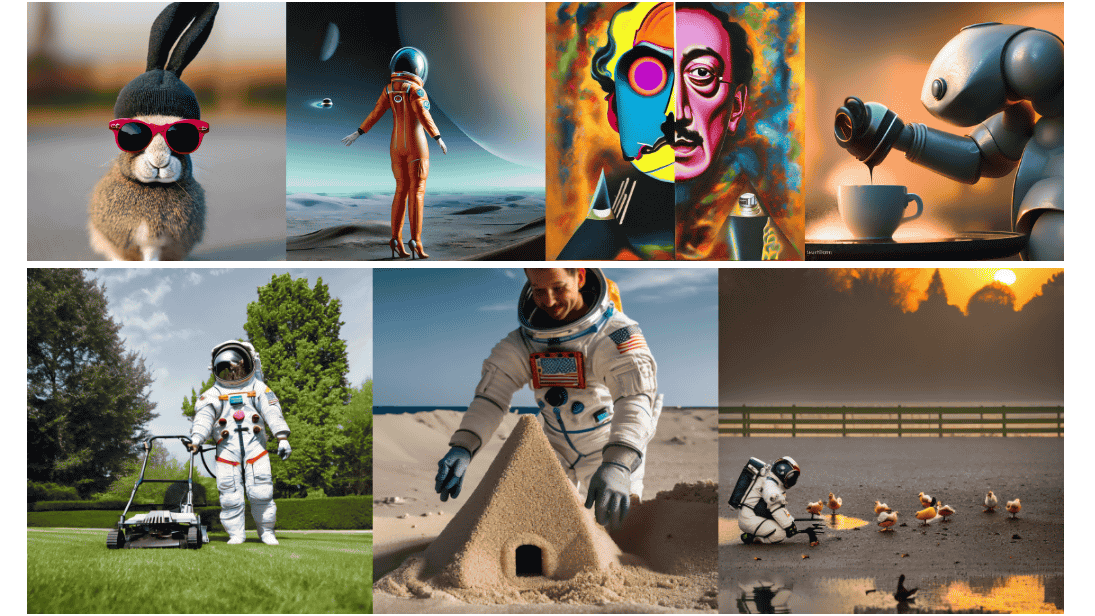
As we dive deeper into this blog, we’ll explore a particularly exciting class of generative models — diffusion models — which are the core of the stable diffusion solution and uncover how they’re used to create impressive visual outputs
Enters diffusion models
Diffusion models have emerged as a groundbreaking innovation in generative AI, with applications ranging from image generation to audio synthesis. These models gained widespread attention in 2022, powering well-known tools like DALL·E 2 and Google’s Imagen, reshaping the landscape of creative AI.
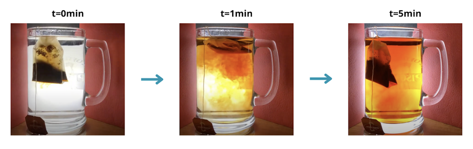
At their core, diffusion models borrow inspiration from non-equilibrium thermodynamics, particularly the concept of diffusion. But don’t worry — we’re not here to dive into a physics lecture! However, understanding the analogy helps clarify how these models work. Think of it like this: when you drop a tea bag into a cup of hot water, the tea’s molecules diffuse from an area of high concentration (the tea bag) into the water, gradually spreading and changing the color of the water. This diffusion process eventually leads to an equilibrium state, where the tea is evenly distributed throughout the water.
Now, in the case of diffusion models, the idea is similar but applied to data like images or audio. The “information” at the start — think of a crisp image or a clean sound sample — undergoes a forward process where noise is gradually added, akin to the tea molecules spreading into the water. As this process continues, the input data becomes increasingly noisy, losing more and more of its recognizable features.
The magic of diffusion models lies in their ability to reverse this process. Just as it would be impossible to “undo” the tea diffusion in water, these models aim to reverse the diffusion process in data. By learning how to add and remove noise at each step, diffusion models can generate new, high-quality samples from a noisy starting point, whether it’s reconstructing an image or generating entirely new content.
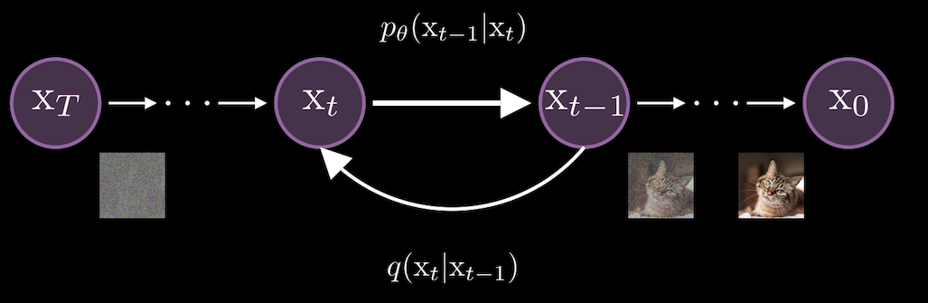
In technical terms, diffusion models work by gradually adding noise to data in a series of steps, modeled by a process called a Markov chain. At each step, a small amount of noise is applied to the input, moving from a clear image, or data point, to a fully noisy version. This is known as the forward process and is represented as \(q(x_t∣x_{t−1})\), where each step \(t\) depends on the previous step \(t−1\).
The goal during training is to learn the reverse process, \(p_\theta(x_{t−1}∣x_t)\), which gradually removes the noise added in the forward steps.
Equations… A lot of Equations!
Now, let’s dive into the mathematics. Don’t worry if the equations seem complex at first—grasping the intuition behind them will make things much easier to follow.
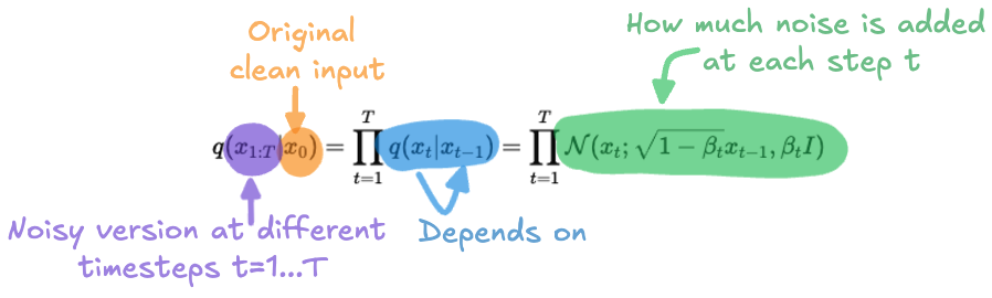
First, we define the forward process, where noise is progressively added to the input data:
Now, the goal of the reverse process is to undo this destruction, starting from noise and gradually “denoising” the data to recover the original clean image:
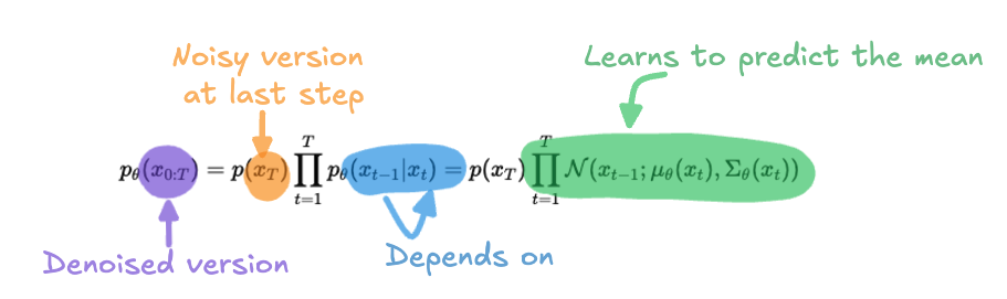
The reverse process learns to predict \(x_{t−1}\) based on \(x_t\). Instead of explicitly specifying the mean and variance, the model is trained to predict the mean \(\mu_\theta(x_t)\), which helps recover the denoised version of the data at each step. The variance \(\Sigma_\theta(x_t)\) is typically fixed to simplify the computation, as it’s assumed to follow a Gaussian distribution.

Visualizing this pipeline, you might be wondering how the model generates an image when you only provide a text prompt, as seen in various applications. In this scenario, the process starts with an image—but not just any image. It’s pure noise, essentially a canvas of random pixels. The model then refines this noisy image step by step, guided entirely by the text prompt you provide. This technique, known as classifier-free guidance, ensures that the generated image aligns closely with the meaning and context of the text. We’ll dive deeper into how this guidance works shortly.
Going back now to the maths behind diffusion models. As seen previously, these models have two steps: a forward process and a backward process. The goal of training a diffusion model is to find the reverse Markov transitions that maximize the likelihood of the training data. In other words, the model learns to predict the noise that was added to \(x_{t-1}\) to turn it into \(x_t\). The objective is to make the predicted noise as close as possible to the real noise added. More generally, training is achieved by optimizing the variational bound on the negative log-likelihood (NLL).
This might look complex at first glance, but let’s break it down step-by-step. The model’s goal is to learn the parameters required to reverse the noise-adding Markov process. Ideally, we would maximize the likelihood of the true distribution over our dataset, \(\log p_\theta(x_0)\). However, directly maximizing this likelihood is practically infeasible due to the high computational cost involved. This is what we call an intractable problem.
To make this optimization feasible, we instead find a lower bound to this likelihood and maximize it. Maximizing this lower bound indirectly maximizes \(\log p_\theta(x_0)\), achieving our goal. This approach is known as the Evidence Lower Bound (ELBO), defined as:
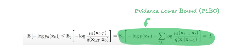
Think of this with an analogy: imagine you own a company where your total revenue comes from multiple sources like sales, investments, and partnerships. Since your total revenue is the sum of all these channels, any individual channel, like sales, represents a lower bound to your total revenue. If you focus on maximizing sales, your total revenue will increase indirectly. Similarly, in training diffusion models, we maximize this lower bound (the ELBO), which indirectly optimizes the true data likelihood.
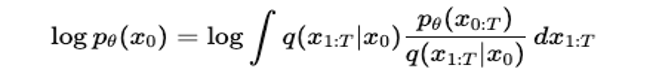
But how do we define this lower bound? A useful starting point is the data distribution from the forward process. By comparing this distribution to the joint distribution over all variables from \(x_0\) to \(x_T\), we can express the log-likelihood of our data distribution as,
Using Jensen’s Inequality, we derive a lower bound by moving the logarithm inside the expectation,
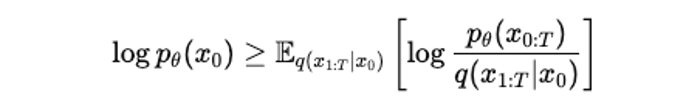
And voilà, we have our lower bound that we can maximize instead. This bound, the ELBO, is what drives our optimization process during training.
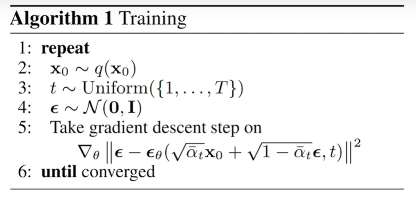
Practically, once we establish the ELBO, we can use it to define the model’s loss function, as shown in step 5 of the training algorithm. In simple terms, the model learns to predict the noise added at each timestep \(t\), given a noisy image of the form \(\sqrt{\bar{\alpha_t}}x_0 + \sqrt{1 - \bar{\alpha_t}}\). Here, \(x_0\) is the original image, and \(\epsilon\) is the added noise sampled from a Gaussian distribution. By performing gradient descent on this loss function, we optimize the model to minimize the difference between the predicted and true noise values. This, in turn, maximizes the ELBO, which indirectly maximizes the likelihood of our data distribution, helping the model learn the reverse process effectively.
Implementation Details
You might be thinking, “Okay… This might be really hard to implement.” But what if I told you that you can get this up in less than 20 lines of code? Let me show you how straightforward it is.
class Diffusion(keras.models.Model):
    def __init__(self):
        super().__init__()
        self.time_embedding = TimeEmbedding(320)
        self.unet = UNET()
        self.final = UNET_OutputLayer(320, 4)

    def call(self, inputs):
        # Inputs:
        # latent: (batch_size, 4, height/8, width/8) - Image latent vector
        # context: (batch_size, seq_len, dim) - Text prompt embedding
        # time: (1, 320) - Time embedding vector
        latent, context, time = inputs

        # Time embedding transformation
        # Maps (1, 320) to (1, 1280) for compatibility with UNET
        time = self.time_embedding(time)

        # Process latent with UNET
        # Input: latent (batch_size, 4, height/8, width/8)
        # Output: processed latent (batch_size, 320, height/8, width/8)
        output = self.unet(latent, context, time)

        # Refine the output for final prediction
        # Maps back to the original latent format: (batch_size, 4, height/8, width/8)
        output = self.final(output)


        return output
That’s it! The heavy lifting here is done by the UNET architecture, which we’ll break down shortly. But before diving into that, let’s unpack what’s happening in this function and why these components are essential.
The diffusion model takes three inputs, each serving a crucial role:
-
Latent Vector - This represents your input image after being processed by the VAE (Variational Autoencoder) encoder. In simpler terms, it’s a compressed representation of your image data.
-
Context - This is the text prompt embedding obtained from the CLIP encoder. It links the text description to the image, guiding the diffusion process toward generating coherent outputs.
-
Timestep - A scalar value embedded as a vector, representing the current step in the denoising process. It helps the model understand when it is in the sequence of removing noise.
Each of these inputs flows through a carefully designed pipeline. The time embedding enriches the model’s understanding of the timestep by transforming it into a higher-dimensional space. Then, the UNET does most of the work: it processes the latent image, guided by the text context and timestep, to refine it at each step of the diffusion process. Finally, the output layer ensures the result is mapped back into the latent space’s original dimensions, ready for further processing or decoding.
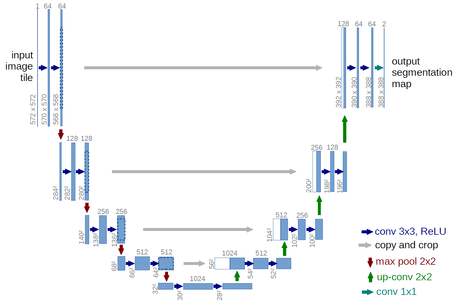
UNET
Now that we’ve explored the training objective of diffusion models—learning to predict and remove noise—let’s look at the architecture that makes this possible. In Stable Diffusion, the model responsible for predicting the noise at each timestep is called UNet.
UNet was originally introduced as an architecture for biomedical image segmentation, designed to handle the challenge of locating fine details in medical images. Moreover, there is a large consent that deep neural networks require many thousand annotated training samples to be performing. UNET is able to perform really well using few annotated samples by leveraging its built in data augmentation, and is relatively fast compared to other methods. Created by Ronneberger et al. in 2015
Stable Diffusion leverages these qualities, repurposing UNet’s structure to predict noise in images. The UNET in stable diffusion takes as input the noisy latent image, produced by the encoder of the VAE, as well as a text prompt and predicts how much noise was added to the latent image, which is the difference between a less noisy image and the input image. The process is used for Denoising Diffusion Probabilistic Models (DDPM) type diffusion models, another approach using the gradient between two steps is used in a score-based diffusion model.
The diffusion process consists in taking a noisy latent image and pass it through the UNET several times. The process ends after a given number of steps, and the output image should represent a noiseless image similar to that of the training data. That is the model should learn to remove the noise and produce an almost exact image as the one of the training data.
We’ve discussed how UNet operates on a noisy image and its role within diffusion models. However, in Stable Diffusion, UNet takes in not only the noisy image but also two additional inputs: the text prompt embedding and the timestep. The text prompt embedding, derived from the CLIP model which we will see later, acts as guidance for the UNet, steering it to generate an image that aligns with the provided text description. Meanwhile, the timestep indicates the amount of noise present at each step, helping the model predict and remove noise more accurately as it moves through the denoising process. These additional inputs enhance UNet’s ability to create high-quality, text-aligned images by combining visual noise reduction with semantic guidance.
Implementation Details
The UNET architecture is the backbone of the diffusion process, responsible for progressively denoising the latent image. It operates in three stages: Input Blocks, a Middle Block, and Output Blocks, connected by skip connections that allow the encoder and decoder to share details. Let’s break it down:
class SpatialTransformer(keras.layers.Layer):
    def __init__(self, channels, n_heads, d_head):
        super().__init__()
        self.norm = keras.layers.GroupNormalization(epsilon=1e-5)
        assert channels == n_heads * d_head
        self.proj_in = PaddedConv2D(n_heads * d_head, kernel_size=1)
        self.transformer_blocks = [BasicTransformerBlock(channels, n_heads, d_head)]
        self.proj_out = PaddedConv2D(channels, kernel_size=1)

    def call(self, inputs):
        x, context = inputs
        b, h, w, c = x.shape
        x_in = x
        x = self.norm(x)
        x = self.proj_in(x)
        x = tf.reshape(x, (-1, h * w, c))
        for block in self.transformer_blocks:
            x = block([x, context])
        x = tf.reshape(x, (-1, h, w, c))
        return self.proj_out(x) + x_in


class Downsample(keras.layers.Layer):
    def __init__(self, channels):
        super().__init__()
        self.op = PaddedConv2D(channels, 3, strides=2, padding=1)

    def call(self, x):
        return self.op(x)


class Upsample(keras.layers.Layer):
    def __init__(self, channels):
        super().__init__()
        self.ups = keras.layers.UpSampling2D(size=(2, 2))
        self.conv = PaddedConv2D(channels, 3, padding=1)

    def call(self, x):
        x = self.ups(x)
        return self.conv(x)


class UNetModel(keras.models.Model):
    def __init__(self):
        super().__init__()
        self.time_embed = [
            keras.layers.Dense(1280),
            keras.activations.swish,
            keras.layers.Dense(1280),
        ]
        self.input_blocks = [
            [PaddedConv2D(320, kernel_size=3, padding=1)],
            [ResBlock(320, 320), SpatialTransformer(320, 8, 40)],
            [ResBlock(320, 320), SpatialTransformer(320, 8, 40)],
            [Downsample(320)],
            [ResBlock(320, 640), SpatialTransformer(640, 8, 80)],
            [ResBlock(640, 640), SpatialTransformer(640, 8, 80)],
            [Downsample(640)],
            [ResBlock(640, 1280), SpatialTransformer(1280, 8, 160)],
            [ResBlock(1280, 1280), SpatialTransformer(1280, 8, 160)],
            [Downsample(1280)],
            [ResBlock(1280, 1280)],
            [ResBlock(1280, 1280)],
        ]
        self.middle_block = [
            ResBlock(1280, 1280),
            SpatialTransformer(1280, 8, 160),
            ResBlock(1280, 1280),
        ]
        self.output_blocks = [
            [ResBlock(2560, 1280)],
            [ResBlock(2560, 1280)],
            [ResBlock(2560, 1280), Upsample(1280)],
            [ResBlock(2560, 1280), SpatialTransformer(1280, 8, 160)],
            [ResBlock(2560, 1280), SpatialTransformer(1280, 8, 160)],
            [
                ResBlock(1920, 1280),
                SpatialTransformer(1280, 8, 160),
                Upsample(1280),
            ],
            [ResBlock(1920, 640), SpatialTransformer(640, 8, 80)],  # 6
            [ResBlock(1280, 640), SpatialTransformer(640, 8, 80)],
            [
                ResBlock(960, 640),
                SpatialTransformer(640, 8, 80),
                Upsample(640),
            ],
            [ResBlock(960, 320), SpatialTransformer(320, 8, 40)],
            [ResBlock(640, 320), SpatialTransformer(320, 8, 40)],
            [ResBlock(640, 320), SpatialTransformer(320, 8, 40)],
        ]
        self.out = [
            keras.layers.GroupNormalization(epsilon=1e-5),
            keras.activations.swish,
            PaddedConv2D(4, kernel_size=3, padding=1),
        ]

    def call(self, inputs):
        x, t_emb, context = inputs
        emb = apply_seq(t_emb, self.time_embed)

        def apply(x, layer):
            if isinstance(layer, ResBlock):
                x = layer([x, emb])
            elif isinstance(layer, SpatialTransformer):
                x = layer([x, context])
            else:
                x = layer(x)
            return x

        saved_inputs = []
        for b in self.input_blocks:
            for layer in b:
                x = apply(x, layer)
            saved_inputs.append(x)

        for layer in self.middle_block:
            x = apply(x, layer)

        for b in self.output_blocks:
            x = tf.concat([x, saved_inputs.pop()], axis=-1)
            for layer in b:
                x = apply(x, layer)
        return apply_seq(x, self.out)
Now this might seem like complicated code, but let me walk you through it. UNET operates in three stages:
- Input Block - which encode the input latent features by progressively downsampling the spatial resolution of the image, where each block contains convolution layers
PaddedConv2D for feature extraction, residual blocksResBlock ,SpatialTransformer to apply Cross-attention since we have different inputs (image, text) and finallyDownsample to reduce feature map resolution. - Middle Block - which is the bottleneck of the network, consisting of 2
ResBlock and aSpatialTransformer - Output_blocks - which decode the features back to the original spatial resolution. There are two additional steps in the code:
- Time Embedding - The timestep embedding is transformed into a feature vector (1280 dimensions) through dense layers and a swish activation to condition the model on the denoising step.
- Final Output - The final block normalizes and refines the output feature map before projecting it back to the latent space dimensions (4 channels) using a
PaddedConv2D .
Classifier-free guidance
Recall that the goal of a diffusion model is to learn \(p_\theta(x)\), the distribution over the training data. However, this function alone doesn’t incorporate additional information, such as a text prompt. In other words, while the model learns to generate images similar to the training data, it doesn’t understand the link between a text prompt, like “a cat” or “a mountain”, and the image generated. To address this, we need a way for the text prompt to serve as a conditioning signal, guiding image generation.
One straightforward solution could be to train the model to learn a joint distribution over the data and the prompt \(c\), i.e., \(p_\theta(x, c)\). However, this approach would require the model to heavily rely on the prompt context, which could risk losing its ability to generate diverse images and would require training a separate model for each conditioning signal, which is inefficient. So, the challenge becomes: how can we make sure the model learns both \(p_\theta(x)\) on its own and while conditioned on the prompt?
Classifier-free guidance offers an elegant solution. Instead of using separate models for conditioned and unconditioned data, we use a single model and occasionally drop the prompt signal. At each timestep, the model receives either the noisy image, the timestep, and the prompt to predict the noise to remove (conditioned case), or the noisy image and timestep without the prompt (unconditioned case). This way, the model learns both to generate images aligned with the prompt and without it.
To guide generation, we combine the two outputs (conditioned and unconditioned) with a weighting factor that controls the degree of conditioning. This weighting is similar to the temperature parameter you might encounter in generative models: the higher the weight given to the prompt, the closer the output will be to the prompt’s description, and the lower the weight, the less influence the prompt has. The final output is calculated as:
\[\text{output} = w * (\text{output}_\text{conditioned} - \text{output}_\text{unconditioned}) + \text{output}_\text{unconditioned}\]This approach allows for fine control over how strongly the prompt influences the generated image, making it a versatile and efficient way to incorporate conditioning into diffusion models.
CLIP
Contrastive Language–Image Pretraining (CLIP) marks a significant advance in multimodal learning. Developed by OpenAI in 2021, CLIP was designed to bridge visual and textual representations, making it possible for models to understand images by being instructed with natural language. Unlike earlier approaches, CLIP enables models to perform a wide range of classification tasks without direct optimization for each task—a concept similar to “zero-shot” learning. Before CLIP, models typically excelled at recognizing specific objects or features but struggled with open-ended prompts, such as understanding the subtle differences between a “sunset on the beach” and a “sunset in the mountains.”
During training, CLIP was exposed to paired images and captions, learning to associate them by embedding both into a shared vector space. Instead of predicting specific labels, CLIP’s training taught it to relate images with descriptive text based on content, allowing it to generalize across a vast range of prompts and contexts.
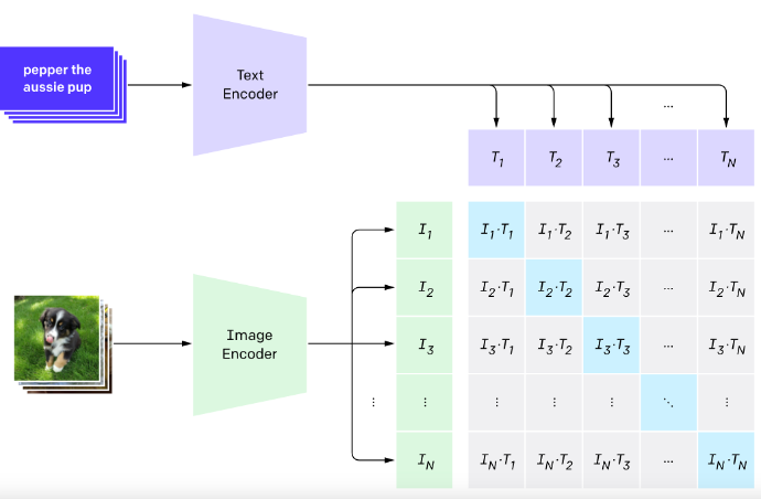
In Stable Diffusion, only the text encoder part of CLIP is used. When given a prompt like “a futuristic cityscape at sunset,” the CLIP encoder transforms this text into an embedding, a numerical representation of the prompt’s meaning. This text embedding serves as a conditioning signal that guides the UNet model in Stable Diffusion, aligning the generated image with the user’s description.
Implementation
As mentioned previously, The CLIP Text Encoder is the backbone of how Stable Diffusion understands and processes text prompts. At its core, it converts a sequence of words into a dense vector or embedding that captures the semantic meaning of the text. This embedding is then used to guide the image generation process.
class ClipTextEmbeddings(keras.layers.Layer):
    def __init__(self, n_vocab, n_embd, n_tokens):
        super().__init__()
        self.token_embedding = keras.layers.Embedding(n_vocab, n_embd)
        self.position_embedding = keras.layers.Embedding(n_tokens, n_embd)

    def call(self, inputs):
        # (batch_size, Seq_len) -> (batch_size, Seq_len, dim)
        input_ids, position_ids = inputs
        word_embeds = self.token_embedding(input_ids)
        pos_embeds = self.position_embedding(position_ids)
        return word_embeds + pos_embeds

class ClipEncoderLayer(keras.layers.Layer):
    def __init__(self, n_head, n_embd):
        super().__init__()
        self.layer_norm_1 = keras.layers.LayerNormalization(epsilon=1e-5)
        self.self_attn = CLIPAttention(n_head, n_embd)
        self.layer_norm_2 = keras.layers.LayerNormalization(epsilon=1e-5)
        self.fc1 = keras.layers.Dense(4 * n_embd)
        self.fc2 = keras.layers.Dense(n_embd)

    def call(self, inputs):
        #(batch_size, Seq_Len, dim)
        # Self attention
        z, causal_attention_mask = inputs
        residue = z
        z = self.layer_norm_1(z)
        z = self.self_attn([z, causal_attention_mask])
        z += residue

        # Feed Forward Layer
        residue = z
        z = self.layer_norm_2(z)
        z = self.fc1(z)
        z = z * tf.sigmoid(1.702 * z) # QuickGelu activation function
        z = self.fc2(z)
        z += residue
        return z

class ClipEncoder(keras.layers.Layer):
    def __init__(self):
        super().__init__()
        self.layers = [ClipEncoderLayer(12,768) for i in range(12)]

    def call(self, inputs):
        [hidden_states, causal_attention_mask] = inputs
        for l in self.layers:
            hidden_states = l([hidden_states, causal_attention_mask])
        return hidden_states

class ClipTextTransformer(keras.models.Model):
    def __init__(self):
        super().__init__()
        self.embeddings = ClipTextEmbeddings(49408, 768, 77)
        self.encoder = ClipEncoder()
        self.final_layer_norm = keras.layers.LayerNormalization(epsilon=1e-5)
        self.causal_attention_mask = tf.constant(
            np.triu(np.ones((1, 1, 77, 77), dtype="float32") * -np.inf, k=1)
        )

    def call(self, inputs):
        # tokens = keras.ops.cast(tokens, tf.int64)
        # (batch_size, Seq_Len) -> (Batch_size, Seq_Len, Dim)
        input_ids, position_ids = inputs
        x = self.embeddings([input_ids, position_ids])
        x = self.encoder([x, self.causal_attention_mask])
        return self.final_layer_norm(x)
The main class,
- The first step is converting the input text or tokens into numerical embeddings. This is done using the class
ClipTextEmbeddings , which combines token embedding and position embedding that adds information about the position of each token in the sequence. - Once the embeddings are ready, they are passed through multiple layers of a transformer encoder
ClipEncoder . This encoder has two main componenents; self-attention and feed-forward networks - Finally, the output is normalized to ensure consistent embedding representations.
Wrap-Up: Bringing It All Together
Stable Diffusion is more than just an impressive tool for generating art—it’s a convergence of years of research into convolutional networks, attention mechanisms, and generative modeling. In this blog series, we’ve carefully unpacked the building blocks of Stable Diffusion, stage by stage, explaining key concepts like convolutions, attention mechanisms, VAEs, and the innovations behind diffusion models. Each section has been designed to give you a solid understanding of these foundations, bridging theory with practical insights.
Through the series, we’ve explored the individual stages of the Stable Diffusion pipeline in detail, from how text is encoded into meaningful representations, to how noisy latents are progressively refined into coherent, high-quality images. For those eager to see how all these pieces fit together into the complete pipeline, the full implementation can be explored through the provided code in the next section. These resources will allow you to follow along, experiment, and build on what you’ve learned.
What’s Next?
The full pipeline implementation in TensorFlow is waiting for you here and the PyTorch implementation here.
Stable Diffusion is a testament to how far AI has come—and where it’s headed. By mastering its foundations, you’re stepping into a world of infinite creativity and innovation. So, grab the code, start experimenting, and let your creativity flow.
Here’s to building the future—one diffusion step at a time!
Here are some more articles you might like to read next: