Stable Diffusion Series 2/5 - Convolution Layers Explained
Understand the role of convolutional layers in the architecture of Stable Diffusion models.
A brief history and why we need it
In the early days of computer vision, researchers faced a significant challenge: how to enable machines to understand and process images as humans do. Traditional neural networks, struggled when applied to images. The main issue was the sheer complexity of visual data—images are high-dimensional, For example a single \(100\times100\)-pixel image has 10,000 pixels, and let us suppose the first layer of the traditional neural network has 512 neurons, that is a total of more than 5 million parameters, this combined with lack of sufficient computational power made the task of computer vision difficult.
Enter convolutional neural networks (CNNs), a groundbreaking approach that revolutionized how we process visual data. The concept of convolution itself isn’t new; it’s a mathematical operation that has been used for decades. However, its application in neural networks was a game changer.
It was in 1998, that LeCun et al. introduced the famous LeNet-5 architecture
What “Convolution” stands for in Convolution Neural Nets
Imagine you’re given two lists of numbers and asked to produce a third list based on these inputs. There are many operations you might consider—element-wise multiplication, addition, or subtraction. Another powerful operation is convolution. But what exactly does that mean? Let’s start by showing the convolution formula and break it down.
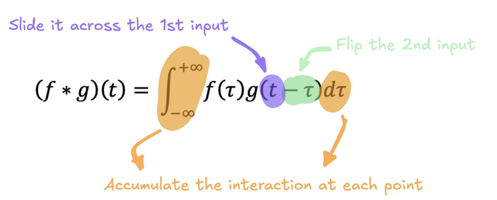
At first glance, this might look intimidating, but don’t worry—math is just a language for describing concepts. In simple terms, to convolve two inputs, f and g, you flip the second input, slide it across the first input, and accumulate the interactions between them at each position.
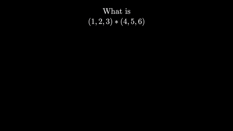
So how does this relate to our example of two lists of numbers? Well, \(f\) and \(g\) can represent those lists. Still not clear? Let’s visualize it with an animation showing the convolution between two lists, \(a\) and \(b\).
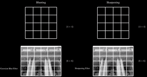
In a convolutional neural network, the input image of shape (height, width) is divided into smaller regions, each of shape (region height,region width). A matrix, called a filter or kernel (we will talk about it later), slides across these regions and applies the convolution operation we just discussed, producing a new layer called a convolutional layer. Instead of each neuron in this layer being connected to every pixel in the input image, it’s connected only to the pixels within its specific region—known as its receptive field.
As you stack more convolutional layers, neurons in each layer connect to small regions of the previous layer, creating a hierarchical structure. This hierarchy allows CNNs to efficiently capture important features in an image, making them incredibly effective for tasks like image recognition.
Technically, we say that a neuron in row \(i\), column \(j\) of a given layer is connected to the outputs of the convolution of neurons in the previous layer located in rows \(i\) to \(i+f_h-1\) and columns \(j\) to \(j+f_w-1\). Where \(f_w\) and \(f_h\) are the width and height of the filter.
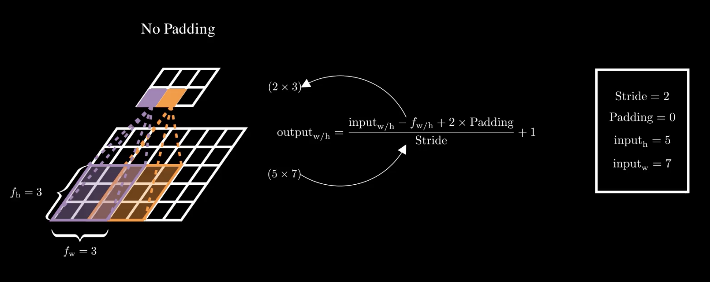
You might notice that with each convolution, the layers tend to shrink in size. If we want to maintain the same height and width as the previous layer, we add zeros around the input—this is known as zero padding.
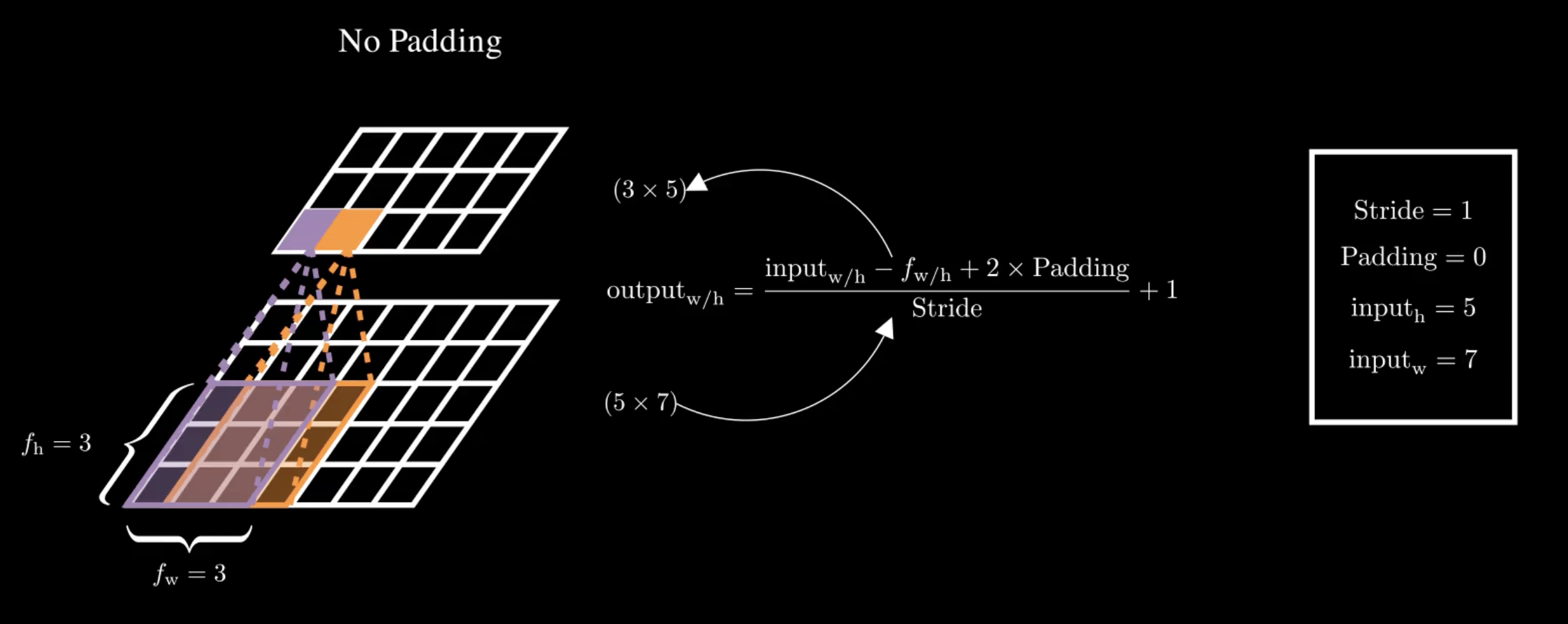
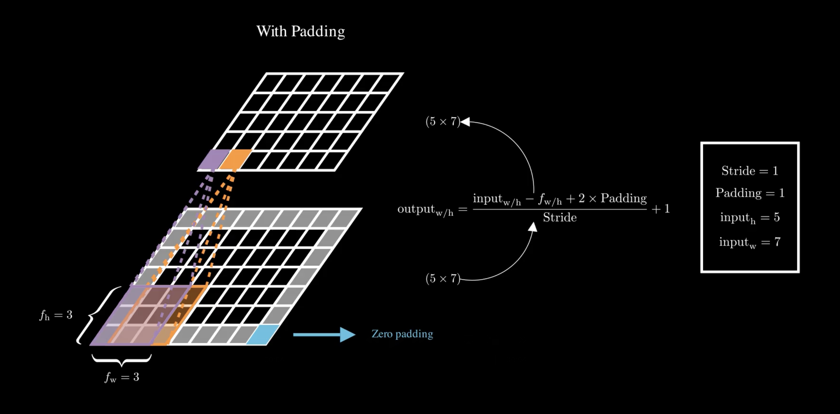
On the other hand, if we want the output to be much smaller, we can space out the positions where we apply the filter. The distance between the current position and the next position of the filter is called the stride.
Filters
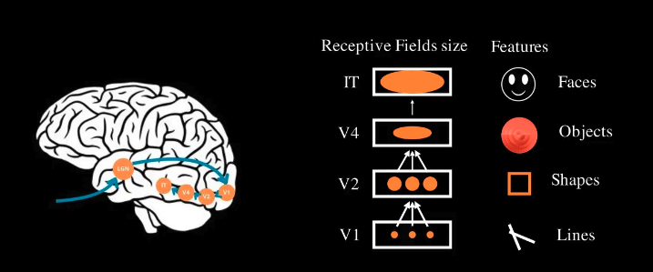
Now, we’ve been talking about filters without introducing them. Simply put, Filters in CNNs play a role similar to that of weights in traditional Artificial Neural Networks (ANN). In an ANN, weights are learned parameters that define the influence of each input feature on the output. Similarly, in a CNN, filters are learned during training and define how different features, such as edges, textures, or shapes, are detected and emphasized in the input image. These filters function much like the receptive fields in the human brain, where each one is responsible for identifying specific features within an image.
What’s particularly powerful about CNNs is that these filters don’t need to be manually defined. Instead, they are automatically learned during the training process through backpropagation and optimization. This means the network discovers the most effective filters for the task at hand, allowing it to efficiently extract meaningful patterns from images.
When a filter slides over an input image, the result is called a feature map. So far, we’ve considered examples with just one filter for simplicity, but in practice, a convolutional layer contains multiple filters, each producing its own feature map.
What sets CNNs apart from traditional ANNs is their ability to detect features regardless of their position in the input. In a CNN, once a feature — like a specific edge or texture — is learned, it can be recognized anywhere in the image. On the other hand, an ANN can only recognize a pattern if it appears in the exact location where it was learned during training. This position-invariance makes CNNs far more efficient, not only in detecting patterns but also in significantly reducing the number of parameters needed, leading to more manageable and effective models.
Convolution layer equation
All the previous explanations would allow us now to easily understand the general equation of a neuron in convolution layer. It is written as follows:
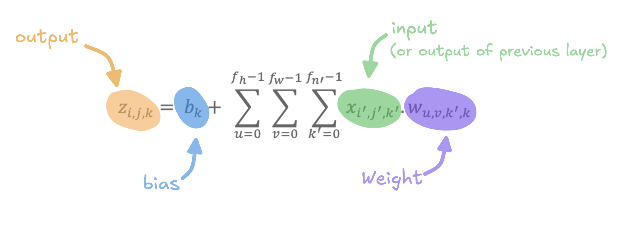
The equation shown in the image represents the computation of the output value \(𝑧_{𝑖,𝑗,𝑘}\) for a single neuron in a convolutional layer of a neural network. Here’s a step-by-step explanation:
- Output \(𝑧_{𝑖,𝑗,𝑘}\) - This is the value of the neuron located in row \(i\) column \(j\), and feature map \(k\) in the current convolutional layer. It represents the activation of this neuron after the convolution operation.
- Input \(x_{𝑖',𝑗',𝑘'}\) - This is the output from the previous layer (or the input image if this is the first layer), specifically from row \(i'\), column \(j'\) and feature map \(k'\).
- Weights \(w_{u,v,k,𝑘'}\) - These are the filter weights applied during convolution. Each weight connects a specific input from a receptive field to the current neuron. The indices \(u\) and \(v\) refer to the position within the receptive field.
- bias \(b_k\) - Each feature map \(k\) has an associated bias term. It adjusts the output of the entire feature map.
The equation sums over \(u\) and \(v\) which correspond to all positions in the receptive field of the input, as well as \(k'\), corresponding to all feature maps.
Implementation
Now that we’ve covered the theory behind convolution, let’s dive into how to implement a convolutional layer in TensorFlow. Fortunately, we don’t need to manually define or compute the convolution operation. TensorFlow provides a convenient Conv2D class that does the heavy lifting for us.
Let’s consider an example input image with the shape \((1, 64, 64, 3)\). Here’s what this shape means:
- The first dimension, \(1\), is the batch size, indicating that we have a single image.
- The next two dimensions, \(64, 64\), represent the height and width of the image.
- The final dimension, \(3\), represents the number of color channels. For an RGB image, there are three channels: red, green, and blue. For grayscale images, this value would be 1.
With that in mind, here’s how we define a convolutional layer in TensorFlow:
  import tensorflow as tf

  # Define a convolutional layer
  conv_layer = tf.keras.layers.Conv2D(
    filters=32,                   # Number of filters
    kernel_size=(3, 3),           # Size of each filter
    strides=(1, 1),               # Stride of the sliding window
    padding='same',               # Padding strategy
    data_format='channels_last'   # Input data format
  )

  # Example input: a batch of images with shape
  # (batch_size, height, width, channels)
  input_tensor = tf.random.normal([1, 64, 64, 3]) # A single 64x64 RGB image

  # Apply the convolution
  output = conv_layer(input_tensor)
  print(output.shape)
This code snippet creates a convolutional layer, applies it to a random RGB image, and prints the shape of the output feature map. The output shape will depend on the filter size, stride, and padding we’ve defined. Now Let us understand each of the
- Filters - This specifies the number of filters (or receptive fields) the convolutional layer will apply to the input. Each filter detects specific patterns or features in the image, such as edges, corners, or textures. As mentioned earlier, we can stack as many filters as needed, and each one will generate its own feature map.
- Kernel_size - This defines the dimensions of each filter. It can either be a single integer or a tuple. In our case, the filters are \(3\times 3\) matrices, which is a common choice for convolutional layers.
- Strides - The stride determines how far the filter moves across the image at each step. It can be a single integer or a tuple that specifies the stride for the height and width. A stride of \((1, 1)\) means the filter will move one pixel at a time both horizontally and vertically. A higher stride value would cause the filter to move in larger steps, reducing the size of the resulting feature map.
-
Padding - There are two options:
-
valid: No padding is added, which means the output feature map will be smaller than the input.
-
same: Zero-padding is applied evenly around the input to maintain the same height and width in the output feature map. This option is useful when you want the output dimensions to match the input dimensions.
-
- Data_format - This determines the order of the dimensions in the input data. By default, TensorFlow uses
channels_last , where the channels (RGB) come last in the shape (i.e., (batch_size, height, width, channels)). If your input has the channels dimension first, as in (batch_size, channels, height, width), you’d usechannels_first to avoid any shape mismatch errors.
Here are some more articles you might like to read next: