Stable Diffusion Series 3/5 - Attention Mechanisms Explained
Understand the role of attention mechanism in the architecture of Stable Diffusion models.

Introduction
In 1950, Alan Turing proposed the famous Turing Test, challenging machines to exhibit human-like intelligence — particularly in mastering language. He envisioned a chatbot based on hardcoded rules, designed to fool a human interlocutor into believing they were conversing with another human. Today, we stand at a point where Large Language Models (LLMs), like GPT-4o, Llama3, and Mistral, have progressed far beyond Turing’s vision, often outperforming humans in tasks like summarization and translation. But how did we reach this point?
Before LLMs became dominant, earlier architectures, such as Recurrent Neural Networks (RNNs), laid the groundwork. Despite different approaches, these models all shared a core principle: predicting the next word based on previous ones. The more “previous words” or context a model could handle, the better its predictions — something we’ll delve into shortly.
But how can machines even begin to understand human language? The key lies in Embeddings — a technique for transforming words into numerical representations that machines can process.
Tokenization
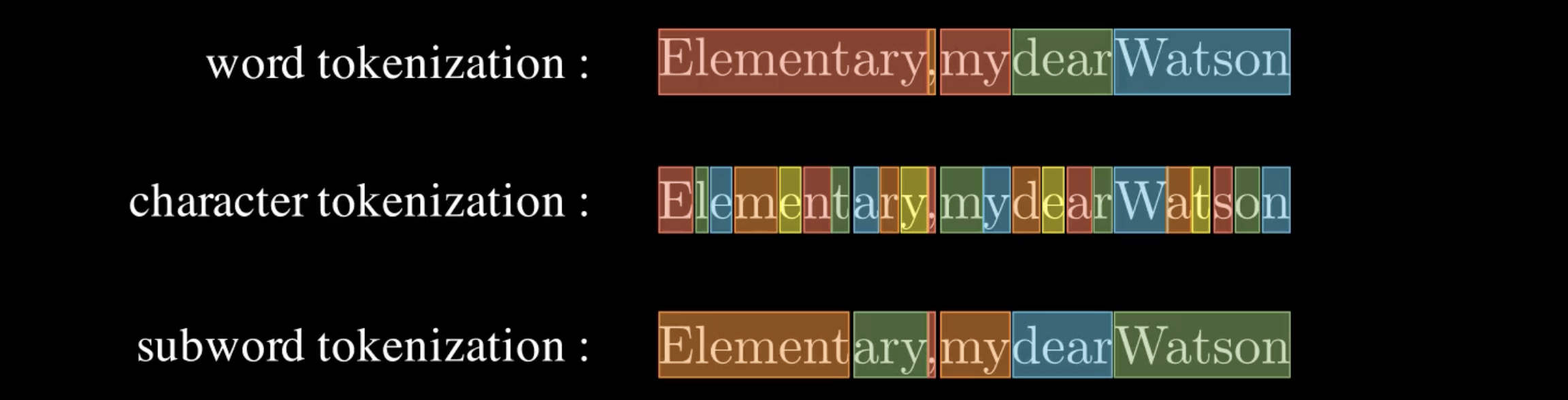
Before discussing embeddings, it’s important to grasp tokenization—the process of breaking down a sentence into smaller units called tokens, which are then converted into embeddings. Tokenization can vary across models, but there are three common methods:
- Word Tokenization - The text is split into individual words.
- Character Tokenization - The text is split into individual characters.
- Subword Tokenization - The text is split into partial words or character sets. This method is commonly used in OpenAI’s GPT models via Byte-Pair Encoding (BPE).
Word embeddings
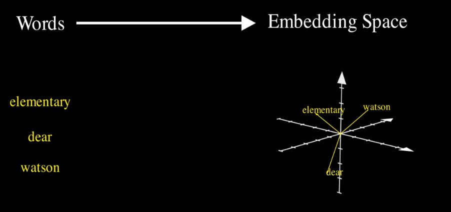
Once a sentence is tokenized, each token is transformed into a vector of floating-point numbers — known as an embedding. These embeddings allow the machine to capture the meaning and relationships between words. For example, the words “elementary,” “dear,” and “Watson” can be represented as vectors in a 3D space:
- “elementary” → [-2, 0, 1]
- “dear” → [-1, 0, -3]
- “Watson” → [2, 0, 2]
This 3D representation is a simplified example. In reality, embeddings used in models like GPT-3 or GPT-4 have much higher dimensions. GPT-3’s embeddings, for instance, span 12,288 dimensions. Such high-dimensional embeddings can’t be visualized, but their purpose remains the same: to represent semantic relationships between words. These embeddings exist within what’s called the embedding space or vector space. In this space, words with similar meanings or relationships are positioned closer together, while words with different meanings are farther apart. For example, the words “king” and “queen” may be positioned near each other due to shared attributes, while “apple” would lie farther away, representing a completely different concept.
As the model trains, it refines these word embeddings to best capture the meanings it learns. Different models have their own unique ways of learning embeddings, but in the case of the transformer architecture, the core architecture of LLMs, embeddings do more than just encode the meaning of individual words. They also include richer information, such as the word’s position in the sentence and its surrounding context.
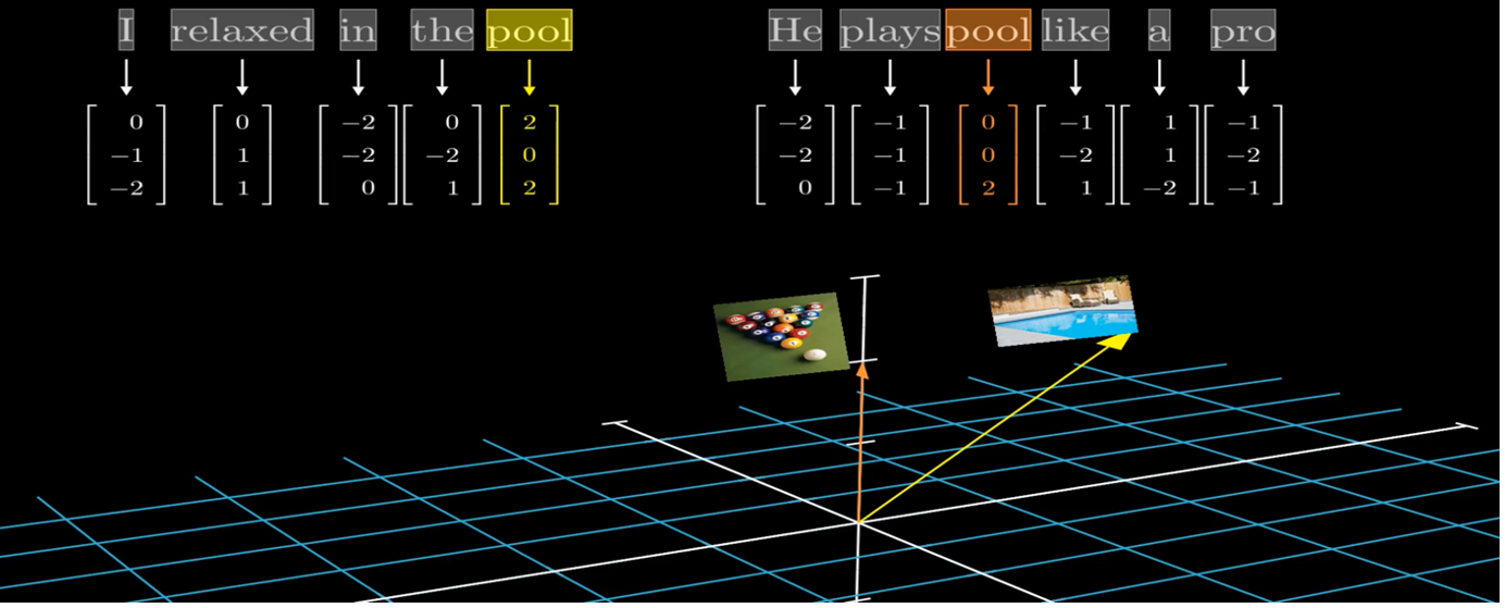
Contextual word embeddings
Language is contextual — words can change their meaning depending on the surrounding words. Transformer models take this into account by adjusting the embedding of a word based on the context in which it appears. The larger the context window, the better the model is at capturing meaning. For example, a model with a 32,000-token context window can consider 32,000 preceding words when generating embeddings for the current word. Naturally, a model with a larger context window performs better than one with a smaller window, as it can “remember” more of the conversation or text.
One way to test this is to compare two models with different context windows: a model with a smaller window will quickly lose track of a long conversation, while a model with a larger window will retain much more context, leading to more coherent responses.
So far, we’ve discussed how embeddings capture the meaning of words in context. But not all words in a context window are equally important. In fact, certain words contribute much more to understanding the meaning of a specific word than others. This is where the Attention mechanism comes into play, a fundamental concept in transformer models. Attention allows the model to focus on the most relevant words in the context, giving more weight to those that are crucial for understanding the current word or token.
How does Attention mechanism work?
The attention mechanism was originally introduced by Dzmitry Bahdanau and colleagues
Over time, several variations of attention have been proposed
To build a deeper intuition for how transformers work, I highly recommend watching Grant Sanderson’s explanation on his YouTube channel, 3Blue1Brown. His visual breakdowns are incredibly insightful.
Now, let’s develop a clear intuition for the attention mechanism before breaking down its underlying mathematics.
Imagine you’re working on a machine translation model, using an encoder-decoder architecture. The encoder processes the input sentence, “I drink milk,” and generates embeddings that represent the sentence’s meaning. The decoder then takes these embeddings and generates the translation, “Je bois du lait.”
During this process, the encoder not only encodes the individual words but also captures the grammatical structure — like recognizing that “I” is the subject and “drink” is the verb. Now, let’s say the decoder has already translated the subject and needs to move on to translating the verb. How does it know which word in the input corresponds to the verb?
It’s helpful to think of the encoder as having created an implicit dictionary like this:
- “subject” → “I”
- “verb” → “drink”
- …
When the decoder is ready to translate the verb, it essentially needs to “look up” the corresponding verb from this dictionary. However, instead of having explicit keys like “subject” or “verb,” the model relies on the embeddings generated by the encoder.
Here’s where attention comes into play. The decoder generates a query, essentially asking, “What part of the input sentence corresponds to the verb I need to translate?” The query is then compared to a set of keys derived from the encoder’s output embeddings. The comparison is done using a similarity measure, specifically the dot-product. The key that most closely matches the query tells the decoder which part of the input to focus on.
Once the attention mechanism identifies the most relevant key, the decoder retrieves the corresponding value, also derived from the encoder’s embeddings, to help generate the next word in the translation.
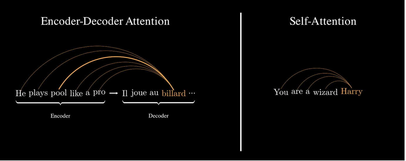
What we have described so far is how the attention mechanism operates in the context of an encoder-decoder architecture. In such models, the encoder processes the entire input sentence and the decoder focuses on specific parts of the encoded representation during translation. However, there’s another type of attention, called self-attention, which is crucial in transformer architectures.
Self-attention operates similarly to the encoder-decoder attention, but with one key difference: instead of focusing on an external sequence, each word in a sentence attends to every other word in the same sentence. This allows the model to build rich contextual representations of each word, accounting for its relationships with all other words in the sequence.
For example, in the sentence “The cat sat on the mat,” the word “cat” would attend to every other word to understand its role in the sentence. This includes attending to “sat” to infer an action associated with the subject and attending to “mat” to identify where the action took place. By doing so, self-attention captures context and dependencies within the sentence more effectively.
Understanding the Scaled Dot-Product Attention
Now that we have an intuition behind the attention mechanism, let’s dive deeper into the Scaled Dot-Product Attention used in transformers. This form of attention is defined mathematically as follows,
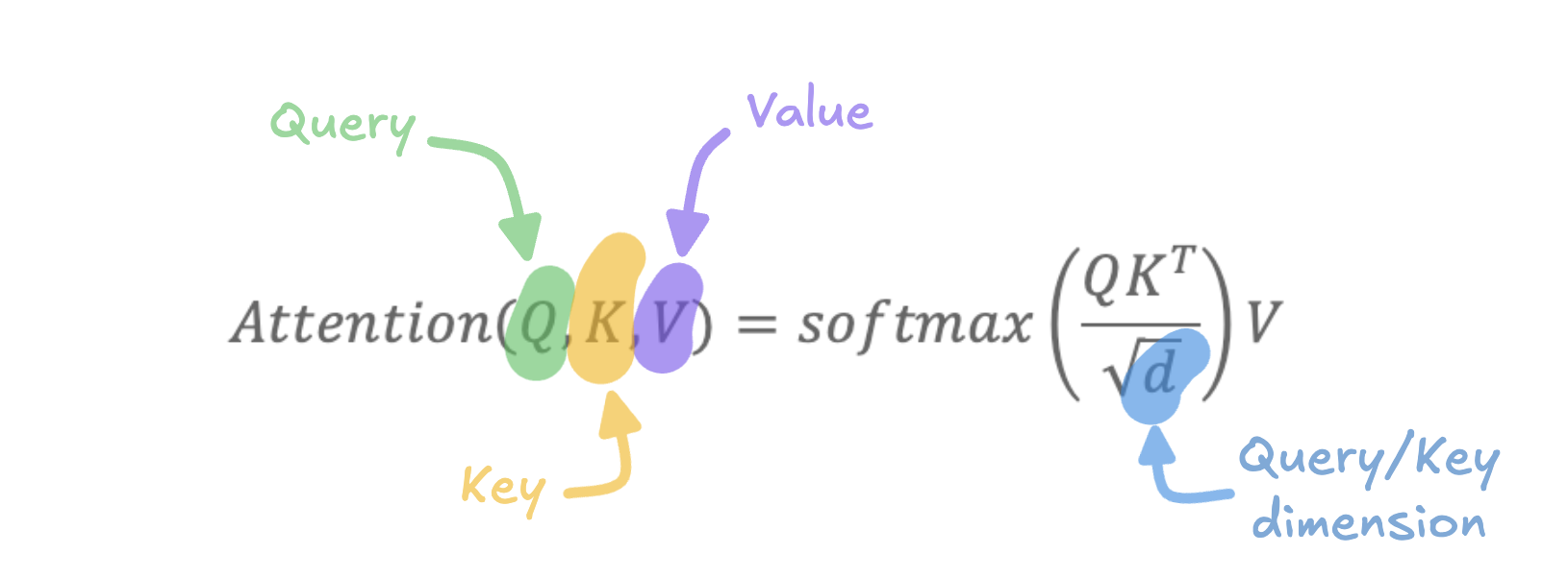
Each matrix is derived by linearly projecting the original token embeddings through learned weight matrices. Let’s break down each component step-by-step:
- Query Matrix \(Q\) - The query matrix is computed by multiplying each token embedding \(E_i\) (at position \(i\)) by a learned weight matrix \(W_Q\). This transformation maps the token embeddings into a new space specifically designed for querying relevant information. The shape of the query matrix is \((n_{queries},d)\),where \(n_{queries}\) is the number of queries (typically equal to the number of tokens in the input) and \(d\) is the dimension of each query vector. For example, in GPT-3, $d$ is 128.
- Key Matrix \(K\) - The key matrix is obtained by multiplying the same token embeddings \(E_i\) by another learned weight matrix \(W_K\). This transformation projects the token embeddings into a new space that is specific to “keys.” Its shape is \((n_{keys},d)\), where \(n_{keys}\) is number of keys and matches the number of queries \(n_{queries}\) in the context of self-attention.
- Dot-product \(QK^T\) - The dot-product between the query and key matrices results in a matrix of shape \((n_{queries},n_{keys})\). Each entry in this matrix represents the similarity score between a query vector and a key vector. Intuitively, if a query closely matches a key, the dot-product will yield a high, positive value. Conversely, if they don’t match, the resulting score will be close to zero or even negative.
- Softmax Normalization - To convert these similarity scores into weights, we apply the softmax function. The softmax operation normalizes the scores such that they sum to 1 along each row, transforming the scores into a probability distribution. This helps the model focus on the most relevant parts of the input while suppressing less important information.
- Scaling by \(\sqrt{d}\) - The division by \(\sqrt{d}\) is introduced to prevent the dot-product values from growing too large, which can lead to gradients that are either too small or too large during training. This scaling ensures more stable optimization.
- Computing the Attention Weights - The result of applying softmax to \(\frac{QK^T}{\sqrt{d}}\) gives us the attention weights. These weights indicate the importance of each word in the input sentence with respect to the query. In other words, the weights tell us how much each word should contribute to the meaning of the word currently being updated.
- Value Matrix \(V\) - Finally, we use a third weight matrix \(W_V\) to project the token embeddings into the value space, forming the value matrix \(V\). This matrix holds the information that we want to pass on, based on the computed attention weights.
- Weighted Sum of Values - The final step is to compute the weighted sum of the value vectors, using the attention weights as coefficients. This step results in a new representation for each word that incorporates contextual information from all other words in the sentence.
Intuition with an example
Let’s return to our example: the sentence “You are a wizard, Harry”. Suppose we want to understand the word “Harry” better by considering its surrounding context. Initially, the model assigns a random embedding to the word “Harry.” However, when we compute the attention weights, we might find that the word “wizard” has a high relevance score with “Harry.” This means the information from the value vector of “wizard” will be heavily weighted when updating the embedding for “Harry.”
As a result, the new embedding for “Harry” will be influenced mostly by its relationship to “wizard,” enabling the model to understand that “Harry” refers to the fictional character, Harry Potter. This context-aware embedding is what gives attention-based models their power in understanding and generating natural language.
Masking
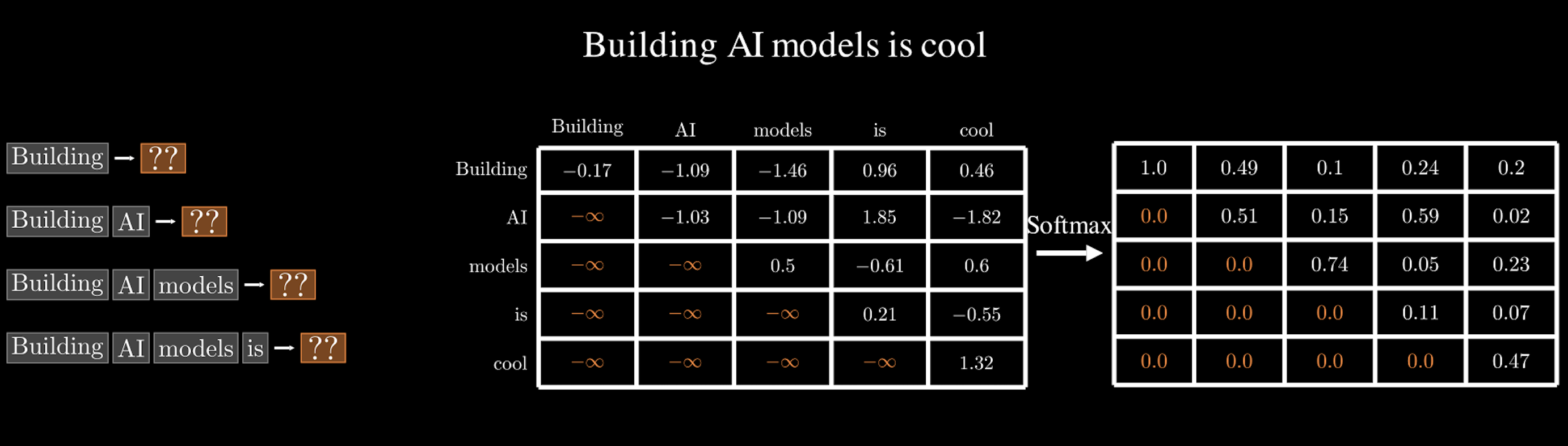
In some cases, we don’t want the model to have access to all the words in a sentence simultaneously. Consider the sentence “Building AI models is cool”. If we want the model to predict the word “AI”, it would be unfair if it could attend to the future words “…models is cool” — essentially giving it access to information it should not yet know. This would be like giving away the answer and would prevent the model from learning proper word dependencies and sequences.
To prevent this, we introduce a technique called masking. Masking allows us to limit the model’s access to certain tokens based on the current context, ensuring that each word prediction only considers the relevant parts of the input.
For example, when predicting the word “AI”, the model should only consider the previous tokens “Building” and not see any of the future words. Similarly, when predicting the next word “models”, it should have access to “Building AI”, but not to “is cool”. This constraint helps the model learn causal relationships and generate text in a step-by-step manner.
How Does it work? The simplest way to implement masking is by modifying the attention weights of future tokens. Specifically, we set these weights to zero, so that the model does not pay any attention to these tokens. This is often achieved by adding a large negative number, typically -\(\infty\) (infinity) to the attention scores of the masked positions before applying the softmax function.
Multi-head Attention
We’re almost at the end of this chapter on attention mechanisms, but there’s one more important concept to cover: multi-head attention.
Multi-head attention is an extension of the scaled dot-product attention mechanism we’ve already discussed. Rather than having just one set of attention weights and outputs, multi-head attention allows the model to use multiple attention mechanisms (or “heads”) in parallel. Each head operates independently and captures different aspects of the input sequence.
Why use multiple attention heads? In the example of using scaled dot-product attention to analyze a sentence, we mentioned that attention can help capture certain grammatical relationships, such as identifying which word is the subject and which is the verb. However, a single head might be limited in what it can represent. It may capture grammatical roles well but miss other nuances like verb tense or semantic relationships between words.
Multi-head attention addresses this limitation by using multiple attention mechanisms in parallel, each focusing on different aspects of the input:
- One head might specialize in capturing grammatical relationships.
- Another head could learn to identify verb tense.
- Yet another might focus on identifying relationships between named entities.
Each head provides a unique “view” of the sentence, allowing the model to understand a richer set of features.
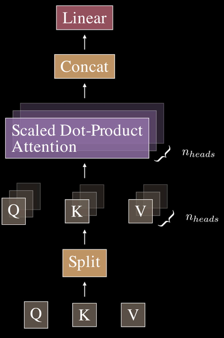
How Does Multi-Head Attention Work? Here’s a step-by-step breakdown of the multi-head attention process: For each token embedding in the input sequence, we apply multiple linear transformations using different sets of learned weight matrices. This results in multiple sets of query, key, and value vectors—one for each head. Each head computes its own scaled dot-product attention using its unique set of query, key, and value vectors. The outputs from all heads are concatenated into a single matrix, combining the unique features learned by each head. Finally, the concatenated output is then passed through a final linear transformation to project it back into the original embedding space.
Implementation
Now, let’s dive into implementing the multi-head attention mechanism. While TensorFlow provides a built-in implementation, we’ll build it from scratch to gain a deeper understanding of its inner workings.
import tensorflow as tf
import numpy as np
import keras
import math

def make_triu(x, dtype=tf.bool):
    """Creates an upper triangular mask for causal attention."""
    ones_like = tf.ones_like(x)
    triu_matrix = tf.linalg.band_part(ones_like, 0, -1)
    result = triu_matrix - tf.linalg.diag(tf.linalg.diag_part(triu_matrix))
    return tf.cast(result, dtype=dtype)

class SelfAttention(keras.layers.Layer):
    def __init__(self, n_heads, d_embd, in_proj_bias=True, out_proj_bias=True):
        super().__init__()
        # Linear layer to project input embeddings into query, key, and value spaces
        self.in_proj = keras.layers.Dense(3 * d_embd, use_bias=in_proj_bias)
        # Linear layer for output projection after attention computation
        self.out_proj = keras.layers.Dense(d_embd, use_bias=out_proj_bias)
        self.n_heads = n_heads  # Number of attention heads
        self.d_head = d_embd // n_heads  # Dimension of each head

    def call(self, inputs, causal_mask=False):
        # Retrieve the input shape: batch size, sequence length, embedding dimension
        input_shape = inputs.shape
        b, s, d_embd = input_shape

        # Reshape intermediate tensors to split dimensions for multi-head attention
        interm_shape = [b, s, self.n_heads, self.d_head]

        # Project input to obtain queries (Q), keys (K), and values (V)
        q, k, v = tf.split(self.in_proj(inputs), 3, axis=-1)  # 3 tensors of shape: (batch_size, seq_len, d_embd)

        # Reshape and transpose Q, K, and V for multi-head attention
        q = tf.transpose(tf.reshape(q, interm_shape), perm=[0, 2, 1, 3])  # (batch_size, n_heads, seq_len, d_head)
        k = tf.transpose(tf.reshape(k, interm_shape), perm=[0, 2, 1, 3])
        v = tf.transpose(tf.reshape(v, interm_shape), perm=[0, 2, 1, 3])

        # Compute attention weights by taking the dot product of Q and K^T
        weight = q @ tf.transpose(k, perm=[0, 1, 3, 2])  # (batch_size, n_heads, seq_len, seq_len)

        # Apply a causal mask if required (used for autoregressive models)
        if causal_mask:
            mask = make_triu(weight, dtype=tf.bool)
            weight = tf.where(mask, -np.inf, weight)  # Mask future tokens by setting scores to -inf

        # Scale weights by the square root of the head dimension for stability
        weight /= math.sqrt(self.d_head)

        # Apply softmax to normalize the weights along the last axis
        weight = tf.nn.softmax(weight, axis=-1)  # Attention probabilities

        # Compute the weighted sum of values (V) based on attention weights
        output = weight @ v  # (batch_size, n_heads, seq_len, d_head)

        # Rearrange and combine multi-head outputs into the original shape
        output = tf.transpose(output, perm=[0, 2, 1, 3])  # (batch_size, seq_len, n_heads, d_head)
        output = tf.reshape(output, input_shape)  # Combine the multi-head dimension

        # Apply the output projection layer
        output = self.out_proj(output)

        return output
The multi-head attention code is divided into 6 main sections:
- Input projection
self.in_proj - This layer projects the input embeddings in a vector space then splits, along the last dimension, the resulting matrix into three separate matrices for queries, keys, and values, required for the attention mechanism. - Multi-head splitting - The queries, keys, and values are reshaped into separate heads. Each head works independently on a smaller dimension
d_head , which improves performance and allows for capturing diverse patterns. - Scaled dot-product attention - The attention score is calculated using the dot product of queries \(Q\) and transposed keys \(K^T\). The result is scaled by the square root of the head dimension to maintain stability during training.
- Causal masking - For autoregressive tasks, this ensures that a token at position \(t\) can only attend to tokens at positions \(\leq t\).
- Attention Application - The softmax function normalizes the scores into probabilities. These probabilities weight the values \(V\) to compute the attention output.
- Output projection
self.out_proj - After combining multi-head outputs into the original embedding space, a dense layer transforms the results back into the desired embedding dimension.
And voilà! Hopefully, this chapter has equipped you with the knowledge to implement and debug an attention mechanism from scratch.
Here are some more articles you might like to read next: